17.11.12

Calibre, Python, reading papers in e-ink

Yesterday I set up the excellent iPython Notebook on my windows machine. This is essentially an interactive web-interface to the Python shell, that lets you record everything you have done, and mark it up with lots of stuff using Markdown and mathjax. In many ways, it is very similar to using RStudio, RMarkdown, and knitr to generate Markdown and html reports from R.

I don't actually do any of my scientific coding in Python, but that may change. My motivation for wanting to learn some Python comes from the fact that Calibre is written in Python. Calibre provides a nice method for taking RSS feeds, parsing them, and spitting out the results as something an e-reader can understand (and really, it supports many different e-reading platforms, including ePub and Kindle formats).

Although I have been using my first generation iPad to read scientific publications from PDF for 2 1/2 years now, the recent experiment of Genome Biology providing the ENCODE publications as ePub made me try reading scientific publications on my 3rd gen Kindle. I loved it! Even without the color figures, and the rather small screen, the experience was simply amazing. Especially given that many papers I am reading more for information intake than for marking up, it really works. And if I really need to mark up a Kindle doc, I can use the Kindle app on my iPad, or my computer. But highlighting works well. I can even retrieve the highlights and notes from the text file that holds them on the Kindle itself.

Most scientific publications are made available as HTML pages, or PDF. So in theory, we should be able to easily generate an ePub or Kindle format using Calibre from the raw HTML. However, for some reason the powers that be in the e-journal publishing world decided that figures and tables should not actually be part of the document. I really don't know why, because they are in the PDF, and it is not that hard to do in the HTML (see an example paper I did here in HTML).

What this ultimately means is that to generate an e-reader compatible document, we need to actually modfiy the HTML. We need to go in, find the elements that tell us where the figure and table pages are, parse them, and get the actual files. I actually figured out how to do this for at least one journal in R using the XML package, and was going to create a package that would take a series of links or DOIs and process them.

But I get many of my papers by RSS feed for specific journals. And Calibre, as I already mentioned, has some nice functions for automatically processing RSS feeds and generating e-reader compatible docs from them. And Calibre is written in Python, and new RSS processing recipes are written in Python. Therefore, I guess I'm going to learn me some Python!

10.10.12

sfLapply vs lapply in R

I've been using the snowfall package for a while to enable parallel processing in R on my Windows machine, where I have an 8 core processor. I discovered today that the function sfLapply will only work with with an object that has a class of list. This is really important, because there are many things that are “list-like”, and are actually lists at heart, but sfLapply probably won't like it.

Lets whip up an example.

require(snowfall)
require(GenomicRanges)

gr <- GRanges(seqnames = Rle(c("chr1", "chr2", "chr1", "chr3"), c(1, 3, 2, 4)), 
    ranges = IRanges(1:10, width = 10:1, names = head(letters, 10)), strand = Rle(strand(c("-", 
        "+", "*", "+", "-")), c(1, 2, 2, 3, 2)), score = 1:10, GC = seq(1, 0, 
        length = 10))

gr
## GRanges with 10 ranges and 2 elementMetadata cols:
##     seqnames    ranges strand |     score                GC
##        <Rle> <IRanges>  <Rle> | <integer>         <numeric>
##   a     chr1  [ 1, 10]      - |         1                 1
##   b     chr2  [ 2, 10]      + |         2 0.888888888888889
##   c     chr2  [ 3, 10]      + |         3 0.777777777777778
##   d     chr2  [ 4, 10]      * |         4 0.666666666666667
##   e     chr1  [ 5, 10]      * |         5 0.555555555555556
##   f     chr1  [ 6, 10]      + |         6 0.444444444444444
##   g     chr3  [ 7, 10]      + |         7 0.333333333333333
##   h     chr3  [ 8, 10]      + |         8 0.222222222222222
##   i     chr3  [ 9, 10]      - |         9 0.111111111111111
##   j     chr3  [10, 10]      - |        10                 0
##   ---
##   seqlengths:
##    chr1 chr2 chr3
##      NA   NA   NA

class(gr)
## [1] "GRanges"
## attr(,"package")
## [1] "GenomicRanges"

grList <- split(gr, seqnames(gr))
grList
## GRangesList of length 3:
## $chr1 
## GRanges with 3 ranges and 2 elementMetadata cols:
##     seqnames    ranges strand |     score                GC
##        <Rle> <IRanges>  <Rle> | <integer>         <numeric>
##   a     chr1   [1, 10]      - |         1                 1
##   e     chr1   [5, 10]      * |         5 0.555555555555556
##   f     chr1   [6, 10]      + |         6 0.444444444444444
## 
## $chr2 
## GRanges with 3 ranges and 2 elementMetadata cols:
##     seqnames  ranges strand | score                GC
##   b     chr2 [2, 10]      + |     2 0.888888888888889
##   c     chr2 [3, 10]      + |     3 0.777777777777778
##   d     chr2 [4, 10]      * |     4 0.666666666666667
## 
## $chr3 
## GRanges with 4 ranges and 2 elementMetadata cols:
##     seqnames   ranges strand | score                GC
##   g     chr3 [ 7, 10]      + |     7 0.333333333333333
##   h     chr3 [ 8, 10]      + |     8 0.222222222222222
##   i     chr3 [ 9, 10]      - |     9 0.111111111111111
##   j     chr3 [10, 10]      - |    10                 0
## 
## ---
## seqlengths:
##  chr1 chr2 chr3
##    NA   NA   NA
class(grList)
## [1] "GRangesList"
## attr(,"package")
## [1] "GenomicRanges"

So we have the GRanges object gr, and a GRangesList in grList. Now lets try to do some parallel execution of finding overlaps of itself.

This is the function we will use in parallel:

returnOverlaps <- function(inObj1, inObj2) {
    findOverlaps(inObj1, inObj2, type = "any")
}
sfInit(parallel = T, cpus = 2)
## Warning: Unknown option on commandline: options(encoding
## R Version:  R version 2.15.0 (2012-03-30)
## snowfall 1.84 initialized (using snow 0.3-10): parallel execution on 2
## CPUs.
sfLibrary(GenomicRanges)
## Library GenomicRanges loaded.
## Library GenomicRanges loaded in cluster.
## Warning: 'keep.source' is deprecated and will be ignored

overlap <- sfLapply(grList, returnOverlaps, gr)
## Error: 2 nodes produced errors; first error: no method for coercing this
## S4 class to a vector

sfStop()
## Stopping cluster

Ok, we get the error no method for coercing this S4 class to a vector. Seems kind of cryptic, at least it did to me. What about using normal lapply?

overlap <- lapply(grList, returnOverlaps, gr)

overlap
## $chr1
## Hits of length 7
## queryLength: 3
## subjectLength: 10
##   queryHits subjectHits 
##    <integer>   <integer> 
##  1         1           1 
##  2         1           5 
##  3         2           1 
##  4         2           5 
##  5         2           6 
##  6         3           5 
##  7         3           6 
## 
## $chr2
## Hits of length 9
## queryLength: 3
## subjectLength: 10
##   queryHits subjectHits 
##    <integer>   <integer> 
##  1         1           2 
##  2         1           3 
##  3         1           4 
##  4         2           2 
##  5         2           3 
##  6         2           4 
##  7         3           2 
##  8         3           3 
##  9         3           4 
## 
## $chr3
## Hits of length 8
## queryLength: 4
## subjectLength: 10
##   queryHits subjectHits 
##    <integer>   <integer> 
##  1         1           7 
##  2         1           8 
##  3         2           7 
##  4         2           8 
##  5         3           9 
##  6         3          10 
##  7         4           9 
##  8         4          10

This works without any errors. Odd. It was only when I was trying to get this to work using llply from the plyr package that I saw a message about as.default.list or something like that. So maybe we have to convert the grList to a good and proper list first?

sfInit(parallel = T, cpus = 2)
## Warning: Unknown option on commandline: options(encoding
## snowfall 1.84 initialized (using snow 0.3-10): parallel execution on 2
## CPUs.
sfLibrary(GenomicRanges)
## Library GenomicRanges loaded.
## Library GenomicRanges loaded in cluster.
## Warning: 'keep.source' is deprecated and will be ignored

grList <- as.list(grList)
overlap2 <- sfLapply(grList, returnOverlaps, gr)

sfStop()
## Stopping cluster

overlap2
## $chr1
## Hits of length 7
## queryLength: 3
## subjectLength: 10
##   queryHits subjectHits 
##    <integer>   <integer> 
##  1         1           1 
##  2         1           5 
##  3         2           1 
##  4         2           5 
##  5         2           6 
##  6         3           5 
##  7         3           6 
## 
## $chr2
## Hits of length 9
## queryLength: 3
## subjectLength: 10
##   queryHits subjectHits 
##    <integer>   <integer> 
##  1         1           2 
##  2         1           3 
##  3         1           4 
##  4         2           2 
##  5         2           3 
##  6         2           4 
##  7         3           2 
##  8         3           3 
##  9         3           4 
## 
## $chr3
## Hits of length 8
## queryLength: 4
## subjectLength: 10
##   queryHits subjectHits 
##    <integer>   <integer> 
##  1         1           7 
##  2         1           8 
##  3         2           7 
##  4         2           8 
##  5         3           9 
##  6         3          10 
##  7         4           9 
##  8         4          10

It works! I'm not exactly sure why there is this difference, but I thought perhaps I can save someone else a few hours time figuring it out.

SessionInfo:

sessionInfo()

R version 2.15.0 (2012-03-30) Platform: x86_64-pc-mingw32/x64 (64-bit)

locale: [1] LC_COLLATE=English_United States.1252 [2] LC_CTYPE=English_United States.1252
[3] LC_MONETARY=English_United States.1252 [4] LC_NUMERIC=C
[5] LC_TIME=English_United States.1252

attached base packages: [1] stats graphics grDevices utils datasets methods base

other attached packages: [1] GenomicRanges_1.8.13 IRanges_1.14.4 BiocGenerics_0.2.0
[4] snowfall_1.84 snow_0.3-10 knitr_0.8.1

loaded via a namespace (and not attached): [1] digest_0.5.2 evaluate_0.4.2 formatR_0.6 plyr_1.7.1
[5] stats4_2.15.0 stringr_0.6.1 tools_2.15.0

Posted on Blogger. Rmd, md

9.10.12

Writing papers using R Markdown

I have been watching the activity in RStudio and knitr for a while, and have even been using Rmd (R markdown) files in my own work as a way to easily provide commentary on an actual dataset analysis. Yihui has proposed writing papers in markdown and posting them to a blog as a way to host a statistics journal, and lots of people are now using knitr as a way to create reproducible blog posts that include code (including yours truly).

The idea of writing a paper that actually includes the necessary code to perform the analysis, and is actually readable in its raw form, and that someone else could actually run was pretty appealing. Unfortunately, I had not had the time or opportunity to actually try it, until recently our group submitted a conference paper that included a lot of analysis in R that seemed like the perfect opportunity to try this. (I will link to the paper here when I hear more, or get clearance from my PI). Originally we wrote the paper in Microsoft® Word, but after submission I decided to see what it would have taken to write it as an Rmd document that could then generate markdown or html.

It turned out that it was not that hard, but it did force me to do some things differently. This is what I want to discuss here.

Advantages

I actually found it much easier to have the text with the analysis (in contrast to having to be separate in a Word document), and upon doing the conversion, discovered some possible numerical errors that crept in because of having to copy numerical results separately (that is the nice thing about being able to insert variable directly into the text). In addition, the Word template for the submission didn't play nice with automatic table and figure numbering, so our table and figure numbering got messed up in the submission. So overall, I'd say it worked out better with the Rmd file overall, even with the having to create functions to handle table and figure numbering properly myself (see below).

Tables and Figures

As I'm sure most of you know, Word (and other WYSIWYG editors) have ability to keep track of your object numbers, this is especially nice for keeping your figure and table numbers straight. Of course, there is no such ability built into a static text file, but I found it was easy to write a couple of functions for this. The way I came up with is to have a variable that contains a label for the figure or table, a function that increments the counter when new figures or tables are added, and a function that prints the associated number for a particular label. This does require a bit of forethought on the part of the writer, because you may have to add a table or figure label to the variable long before you actually create it, but as long as you use sane (i.e. descriptive) labels, it shouldn't be a big deal. Let me show you what I mean.

Counting

incCount <- function(inObj, useName) {
    nObj <- length(inObj)
    useNum <- max(inObj) + 1
    inObj <- c(inObj, useNum)
    names(inObj)[nObj + 1] <- useName
    inObj
}
figCount <- c(`_` = 0)
tableCount <- c(`_` = 0)

The incCount function is very simple, it takes an object, checks the maximum count, and then adds an incremental value with the supplied name. In this example, I initialized the figCount and tableCount objects with a non-sensical named value of zero.

Now in the process of writing, I decide I'm going to need a table on the amount of time spent by post-docs writing blog posts in different years of their post-doc training. Lets call this t.blogPostDocs. Notice that this is a fairly descriptive name. We can assign it a number like so:

tableCount <- incCount(tableCount, "t.blogPostDocs")
tableCount
##              _ t.blogPostDocs 
##              0              1

Inserting

So now we have a variable with a named number we can refer to. But how do we insert it into the text? We are going to use another function that will let us insert either the text with a link, or just the text itself.

pasteLabel <- function(preText, inObj, objName, insLink = TRUE) {
    objNum <- inObj[objName]

    useText <- paste(preText, objNum, sep = " ")
    if (insLink) {
        useText <- paste("[", useText, "](#", objName, ")", sep = "")
    }
    useText
}

This function allows us to insert the table number like so:

r I(pasteLabel("Table", tableCount, "t.blogPostDocs"))

This would be inserted into a normal inline code block. The I makes sure that the text will appear as normal text, and not get formatted as a code block. The default behavior is to insert as a relative link, thereby enabling the use of relative links to link where a table / figure is mentioned to its actual location. For example, we can insert the anchor link like so:

<a id="t.blogPostDocs"></a>

Markdown Tables

Followed by the actual table text. This brings up the subject of markdown tables. I also wrote a function (thanks to Yihui again) that transforms a normal R data.frame to a markdown table.

tableCat <- function(inFrame) {
    outText <- paste(names(inFrame), collapse = " | ")
    outText <- c(outText, paste(rep("---", ncol(inFrame)), collapse = " | "))
    invisible(apply(inFrame, 1, function(inRow) {
        outText <<- c(outText, paste(inRow, collapse = " | "))
    }))
    return(outText)
}

Lets see it in action.

postDocBlogs <- data.frame(PD = c("p1", "p2", "p3"), NBlog = c(4, 10, 2), Year = c(1, 
    4, 2))
postDocBlogs
##   PD NBlog Year
## 1 p1     4    1
## 2 p2    10    4
## 3 p3     2    2

postDocInsert <- tableCat(postDocBlogs)
postDocInsert
## [1] "PD | NBlog | Year" "--- | --- | ---"   "p1 |  4 | 1"      
## [4] "p2 | 10 | 4"       "p3 |  2 | 2"

To actually insert it into the text, use a code chunk with results='asis' and echo=FALSE.

cat(postDocInsert, sep = "\n")
PD NBlog Year
p1 4 1
p2 10 4
p3 2 2

Before inserting the table though, you might want an inline code with the table number and caption, like this:

I(pasteLabel("Table", tableCount, "t.blogPostDocs", FALSE)) This is the number of blog posts and year of training for post-docs.

Table 1 This is the number of blog posts and year of training for post-docs.

Remember for captions to set the insLink variable to FALSE so that you don't generate a link from the caption.

Figures

Oftentimes, you will have code that generates the figure, and then you want to insert the figure at a different point. This is accomplished by the judicious use of echo and include chunk options.

For example, we can create a ggplot2 figure and store it in a variable in one chunk, and then print it in a later chunk to actually insert it into the text body.

plotData <- data.frame(x = rnorm(1000, 1, 5), y = rnorm(1000, 0, 2))
plotKeep <- ggplot(plotData, aes(x = x, y = y)) + geom_point()
figCounts <- incCount(figCount, "f.randomFigure")

And now we decide to actually insert it using print(plotKeep) with the option of echo=FALSE:

plot of chunk figureInsert

Figure 1. A random figure.

Numerical result formatting

When R prints a number, it normally likes to do so with lots of digits. This is not probably what you want either in a table or when reporting a number in a sentence. You can control that by using the format function. When generating a new variable, the number of digits to display when printing will be saved, and when used on a variable directly, only the defined number of digits will display.

Echo and Include

This brings up the issue of how to keep the code from appearing in the text body. I found depending on the particulars, either using echo=FALSE or include=FALSE would do the job. This is meant to be a paper, a reproducible one, but a paper nonetheless, and therefore the code should not end up in the text body.

References

One thing I haven't done yet is convert all the references. I am planning to try using the knitcitations package. I will probably post on that experience.

HTML generation

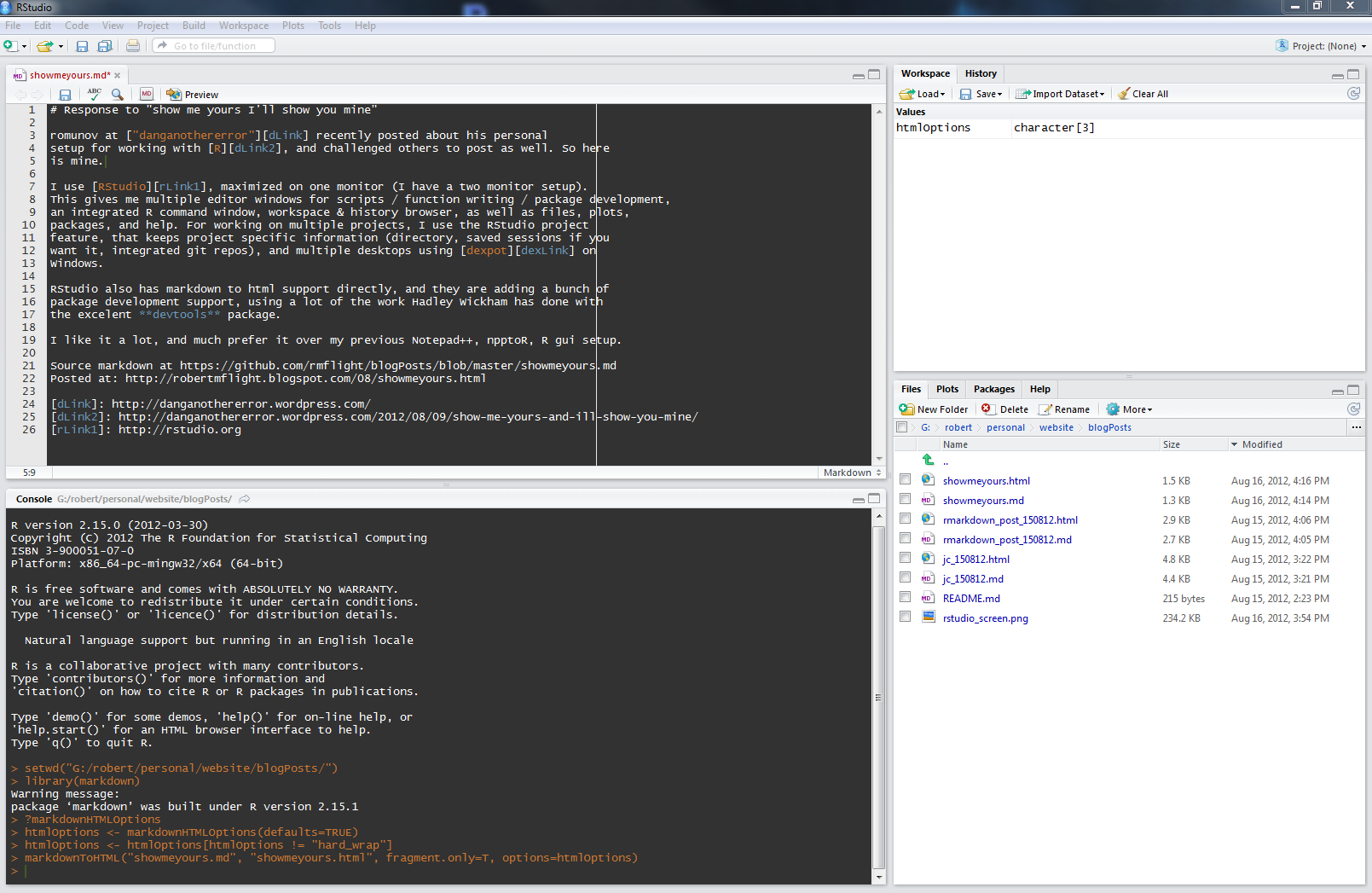
Because I use RStudio, I set up a modified function For generating a full html version of the paper, changing the default RStudio markdown render options like so:

htmlOptions <- markdownHTMLOptions(defaults=TRUE)
htmlOptions <- htmlOptions[htmlOptions != "hard_wrap"]
markdownToHTML(inputFile, outputFile, options = htmlOptions)

This should be added to a .Rprofile file either in your home directory or in the directory you start R in (this is especially useful for modification on a per project basis).

I do this because when I write my documents, I want the source to be readable online. If this is a github hosted repo, that means being displayed in the github file browser, which does not do line wrapping. So I set up a 120 character line in my editor, and try very hard to stick to that.

Function source

You can find the previously mentioned functions in a github gist here.

Post source

The source files for this blog post can be found at: Rmd, md, and html.

Posted on October 9, 2012, at http://robertmflight.blogspot.com/2012/10/writing-papers-using-r-markdown.html

Edit: added section on formatting numerical results

Edit: added session info

R version 2.15.0 (2012-03-30)
Platform: x86_64-pc-mingw32/x64 (64-bit)

locale:
[1] LC_COLLATE=English_United States.1252 
[2] LC_CTYPE=English_United States.1252   
[3] LC_MONETARY=English_United States.1252
[4] LC_NUMERIC=C                          
[5] LC_TIME=English_United States.1252    

attached base packages:
[1] stats     graphics  grDevices utils     datasets  methods   base     

other attached packages:
[1] ggplot2_0.9.2.1 knitr_0.8.1    

loaded via a namespace (and not attached):
 [1] colorspace_1.1-1   dichromat_1.2-4    digest_0.5.2      
 [4] evaluate_0.4.2     formatR_0.6        grid_2.15.0       
 [7] gtable_0.1.1       labeling_0.1       MASS_7.3-21       
[10] memoise_0.1        munsell_0.4        plyr_1.7.1        
[13] proto_0.3-9.2      RColorBrewer_1.0-5 reshape2_1.2.1    
[16] scales_0.2.2       stringr_0.6.1      tools_2.15.0      

12.9.12

AbsIDconvert: New method for converting genomic identifiers

Today our paper “AbsIDconvert: An absolute approach for converting genetic identifiers at different granularities” finally hit BMC Bioinformatics. I'm really excited, because I've been wanting to tell people outside our primary collaborators about it. The website for the tool is http://bioinformatics.louisville.edu/abid. There will eventually be a downloadable virtual machine for local analyses, with no restrictions on the number of items submitted.

The basic premise is that every genetic type of identifier, whether it is an Entrez Gene, Refseq, Ensembl (gene, transcript), and microarray probe (or probeset for Affy) can be reduced to a DNA sequence that can subsequently be placed on a reference genome as a genomic interval. Conversion between different types of identifiers then becomes a problem of finding overlapping genomic intervals.

We have a large number of different types of identifiers for different organisms and genome assemblies stored as genomic intervals, including many Affy and Agilent microarrays. However, if your favorite array is not present, or your identifier doesn't seem to work (as of Sept 12, 2012 there is at least one Agilent array that seems to be missing IDs), you can submit the sequences and find corresponding genomic intervals and translate to other identifiers.

Note that there is a limit on how many sequences / IDs can be uploaded at one time (you will get a message to “Select Genome Version!!!!!!” when you try to upload too many sequences for example). This is removed in the virtual machine version.

The code behind the website uses R, RApache and the GenomicRanges package for storing and querying intervals. Alignment is carried out using Bowtie2

I hope others find this resource (and or approach) useful!

Next week I hope to put up a post with more examples, although you can probably get a good idea of how it works and the possibilities from the publication and the website.

Source hosted at https://github.com/rmflight/blogPosts/blob/master/absidConvert_live.md

Posted to http://robertmflight.blogspot.com/2012/09/absidconvert-new-method-for-converting_12.html

16.8.12

Show me yours

romunov at “danganothererror” recently posted about his personal setup for working with R, and challenged others to post as well. Here is my setup.

I use RStudio, maximized on one monitor (I have a two monitor setup). This gives me multiple editor windows for scripts / function writing / package development, an integrated R command window, workspace & history browser, as well as files, plots, packages, and help. For working on multiple projects, I use the RStudio project feature, that keeps project specific information (directory, saved sessions if you want it, integrated git repos), and multiple desktops using dexpot on Windows.

RStudio also has markdown to html support directly, and they are adding a bunch of package development support, using a lot of the work Hadley Wickham has done with the excelent devtools package.

I like it a lot, and much prefer it over my previous Notepad++, npptoR, R gui setup.

Source markdown at https://github.com/rmflight/blogPosts/blob/master/showmeyours.md

Posted at: http://robertmflight.blogspot.com/2012/08/show-me-yours.html

15.8.12

Loving Markdown!

Ok, so for those who don't know, the guys from RStudio recently teamed up with Yihui to add some really nice report authoring options in RStudio using the packages knitr ability to turn a combination of markdown and R code into html.

I have to admit, this has really changed how I work. Previously, I generally had R scripts, that I would then run, and summarize the results in a separate document as a report on what I had done. I know, many like to talk about Sweave, the language that R uses to generate vignettes demonstrating package functionality, but have you ever tried to write a Sweave document?

You need to know a fair amount about Latex, and even then it can be difficult to get the output you want. In addition, reading the raw file can be quite painful (I know, I have my own Bioconductor package that I wrote a Sweave vignette for).

Writing R Markdown documents just feels different. When I read the raw source of a Markdown document, I can actually read it, code and all. What is really sweet is that instead of writing about what I am doing in the comments, I write it out in full in the document, and then have the code blocks doing the actual calculations. What is really great is to regenerate the report, I simply re-knit it to generate a new html file.

It is so much easier to work with, that I am probably going to switch even how I write my blog posts, using a Markdown document as the source. For right now, that means writing a .md file, and then converting it to html using the R Markdown package, and then writing in the html to Blogger. You can see a good explanation of that process from Jeffrey Horner's blog here and here.

When I combine this with a github repo for storage, it also means I have some other place to keep the raw source of my blog posts, as well as easily read and edit the text. For example, you can read the raw text that was used for this post.

Source of this post is at https://github.com/rmflight/blogPosts/blob/master/rmarkdown_post_150812.md. Published at http://robertmflight.blogspot.com/2012/08/loving-markdown.html

Journal Club: 15.08.12

I just came back from our Bioinformatic group (a rather loose association of various researchers at UofL interested in and doing bioinformatics) journal club, where we discussed this recent paper:

Google Goes Cancer: Improving Outcome Prediction for Cancer Patients by Network-Based Ranking of Marker Genes

Besides the catchy title that makes one believe that perhaps Google is getting into cancer research (maybe they are and we don't know it yet), there were some interesting aspects to this paper.

Premise

The premise is that they can combine gene expression data and network data to find better associations between gene expression data and a particular disease endpoint. The way this is carried out is through the use of the TRANSFAC transcription factor - gene target database for the network, the correlation of the gene expression with the disease status as the importance of a gene with the disease, and the Google PageRank as the means to transfer the network knowledge to the gene expression data. They call their method NetRank.

Note that the general idea had already been tried in this paper on GeneRank.

Implementation

Rank the genes with disease status (poor or good prognosis) using a method (SAM, t-test, fold-change, correlation, NetRank). Pick n top genes, and develop a predictive model using a support vector machine. Wash, rinse, repeat several times to find the best set, varying the number of top genes, and the number of samples used in the training set.

For NetRank, the top genes were decided by using a sub-optimization based on varying d, the dampening factor in the PageRank algorithm that determines how much information can be transferred to other genes. The best value of d determined in this study was 0.3.

All other methods used just the 8000 genes that passed filtering, but NetRank used all the genes on the array, with those that were filtered out had their initial correlations set to 0, so that they were still in the network representation.

Monte Carlo cross-validation

Did it work?

From the paper, it appears to have worked. Using a monte-carlo cross-validation, they were able to achieve over 70% prediction rates. And this was better than any of the other methods they used to associate genes with the disease, including SAM, t-test, fold-change, and raw correlations.

NetRank feature selection performance

Issues

As we discussed the article, some questions did come up.

  1. What was the variation in d depending on the size of the training set?
  2. How consistent were the genes that came out as biomarkers?
    • It would be nice to try this methodology on a series of independent, but related cancer datasets (ie breast or lung cancer) and see how consistent the lists are. This was done here.
  3. What happens if the genes that don't pass filtering are removed from the network entirely?
  4. Were the problems reported with not-filtering genes due to having only two disease points (poor and good prognosis) to calculate a correlation of expression with?
  5. How many iterations does it take to achieve convergence?
  6. The list of genes they come up with are fairly well known cancer genes. We were kindof surprised that they didn't seem to come up novel genes associated directly with pancreatic cancer.
  7. Why is d so variable depending on the cancer examined?

Things to try

  • Could we improve on this by instead of taking just the top-ranked genes, look for the top ranked cliques, i.e. take the top gene, remove anything in its immediate neighborhood, and then go to the next one?
  • What would happen if we used a directed network based on connected Reactome or KEGG pathways?

The markdown source of this post is here.